• The discovery of Carrapateena
• The old & incomplete core logging page

Scale-dependent mapping

This image is based on a figure by Rickard (1892) from an outcrop at Victoria Hill, Bendigo. It shows the influence of vein orientation exploiting lithologically controlled structures. Veins follow bedding (B), axial planar cleavage in shales (A), radial joints in sands (P) and for tension veins (T) related to faults (F).

The important questions are:

• Which of these veins host mineralisation?
• Which veins had access to the mineralised fluids?
• How do the shales act as plugs to trap mineralisation?
• What lithologies are microfractured to host disseminated mineralisation?
• How do you define a resource shape?
• How do you achieve all this from one drill hole?
• What angle do you drill?
• How do the results relate to adjacent drill holes?

Mapping the gold distribution in the shoot is entirely different to mapping out the quartz distribution or to map out the reef. The important job is to integrate the data to delineate the auriferous shoot in three dimensions.

Linex have developed methodologies to achieve detailed stratigraphic and structural reconstructions to achieve these detailed reconstructions.

Rickard, T. A. 1892. The Bendigo gold-field: ore deposits other than saddle reefs, Transactions of the American Institute of Mining Engineers., 21, 686–713.

Methodology

This hypothetical example utilises real data from drill holes logged by differing geologists with differing logging styles (a lumper and a splitter).

The first step is to convert the drilled data to true thickness plots for correlation. Data is aligned and correlated, requiring some cutting and moving around the faults. At this point, the amount of faulted out stratigraphy can be measured which gives a rough idea of fault displacement.

The data can then be correlated on a cross section with the hole traced. The fault position can be drawn in and the dip obtained from beds away from the fault. Infilling the section maintaining the known dip can be achieved where there are no data.

This reconstruction has been made without any structural data and measured structures are important to confirm the validity of and assist with the reconstruction.

An additional step would be to draw in likely vein orientations associated with the faults and differing lithologies to get an idea of likely shoot positions to assist with targeting on the next hole or drill section.

Fosterville Example

Detailed reconstruction of one of multiple drill sections. Several holes on each sections build the stratigraphy and detail and continuity of the structures. Some bizarre faults are revealed by the data that won’t be found in any text book.

The grid on the section is 50m spacing.

The devil is in the detail

For some reason field mapping is rushed and often done by inexperienced geologists. Outcrop provides cheap data to integrate with geophysical data and geochemical data. But if done wrong, it can be horrendously misleading.

These images are the same area mapped by differing geologists. The complex folding has been missed that sheds a completely differing light to the geology and exploration potential of the area.

Modern GPS equipment makes is quick and easy to collect actual data to base interpretations on. In much of Australia, reliable structural readings are difficult to obtain. Following small strike ridges can importantly define bedding trends and the shapes of folds.

Read between the lines and ground truthing

Consider the magnetic blips. How many interpretations have you seen that considers the location (eg flight lines) of the data? How many interpretations have you seen that integrates detailed geology to compare to the data? Most acquire the magnetics and simply interpret that.

In this example, it happened that the overall bedding trend ran parallel to the flight line. But it meandered either side of it. The result is a series of small anomalies.

It is important to know where the data was collected from and how this impacts on the image. You need to read between the lines to adequately interpret the data. A great example, when have you seen a magnetic low by itself and paid no attention to it?

The right tectonic address?

Our tectonic understanding has come a long way in recent years. Recognition of inverted half grabens, toe thrusts and basement transfer faults provides an inherited structural grain and an understanding of the major plumbing faults for mineralisation to access.

Simplified tectonics and fluid access

Jostling of structures over time along a transfer fault creates multiple structures of varying orientation and numerous opportunities for fluid access. The surrounding region may be relatively undeformed.

Geochemical revolution

Where appropriate to utilise, the pXRF has revolutionised field exploration.

In the upper example, the TMI (1VD) image was hypothesised to represent a multi-phase, Porphyry Copper/IRGS target. An initial single loop traverse confirmed the validity of the target and a detail grid was then planned for return the following day. This enables a dynamic and nimble operation to define trends that can be adjusted daily. Multiple areas of high arsenic, a proxy for gold in the district occur and some elevated copper. Confirmation soil sampling was then conducted over target areas to test for gold (laboratory analysis).
Source: Dart Mining

Subtle structures

There is a lot of valuable data waiting to be exploited. Here a pit was never mapped in detail and the key structures shown not identified. A planar hanging wall fault truncates gently flexed beds. The strike difference is barely noticeable on the ground, and small enough to be commonly written of as irrelevant. The intersection of the bedding parallel faults (purple in map view) generated a steeply plunging intersection. This matches the orientation of the shoots on mine plans elsewhere in the goldfield.

Magnetics data – reading between the lines

a) is an example of a magnetic anomaly (assume all data are gridded at the same elevation). I Australia, we typically see a high to the north of a low over a magnetic body.
b) shows what flight line data would record if only 3 lines were flown over the area as shown. c) then would be the gridded result. A high will be plotted, slightly north of where it occurs in reality and no low would be seen.
d) is the scenario where the lines were in a slight differing spot. e) we would get a low with no accompany high.
Line position is critical to image the anomaly and to enable interpretation and modelling. Good interpretation will read between the lines to assess what could be missing.

Gravity data – reading between the data points

Gravity data are collected from stations (points) that can be widely spaced (eg 2 km). a) this example shows 16 widely-spaced stations, four with slightly elevated readings that would be gridded to show 4 separate, insignificant blips. However there is enough room in between for something interesting to happen. b) the addition of a new station reveals a large anomaly in between the four points that only caught the edge of.
Good interpretation will read between the data points to assess what could be missing.

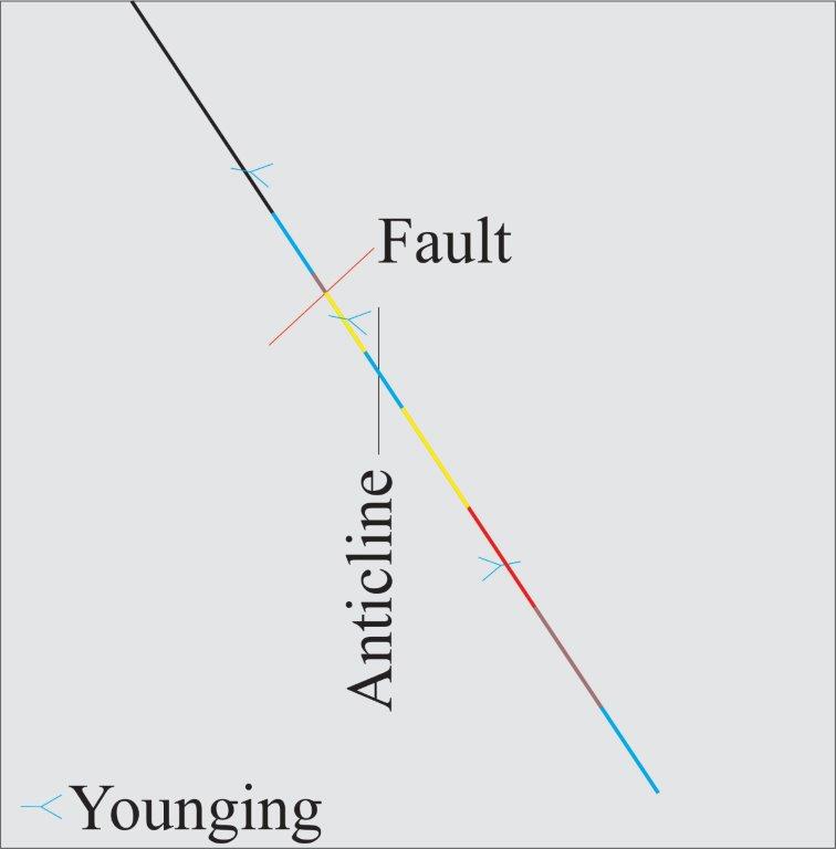
Step 1: Plot key data points on the drill holes

Plot the key domain boundaries & structural details (faults, folds, younging, bedding angles) on the drill section

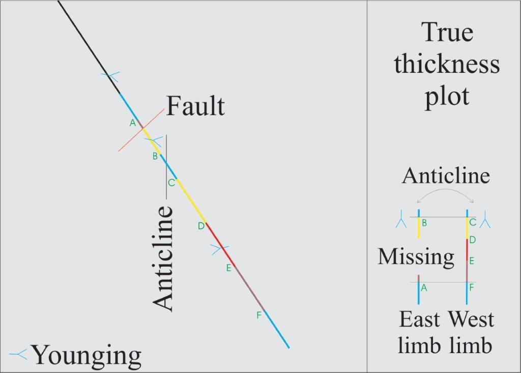
Step 2: Plot correlated marker horizons

Once converted to true thickness, correlate the sediments within each domain. Select key marker horizons. Plot these positions on the drill section.

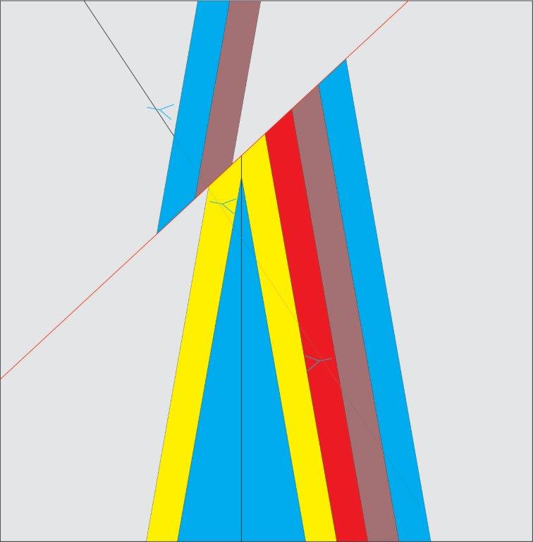
Step 3: Reconstruct data

Using the known dip of the beds, project the key horizons beyond the drill hole. Wrap beds around the folds. This step can often constrain the dip of the axial plan or if any additional faults are offsetting beds.

Step 4: Constrained interpretation

Using the defined stratigraphic thicknesses from Step 2, begin to build the geology away from the drill hole. Once enough stratigraphy has been built, the offset on the fault can be determined, for example using the brown bed on the western limb. The position of the anticline above the fault can then be established and all of the stratigraphy drawn. Often drill targets will be revealed at this stage, for example where the anticline meets the fault.

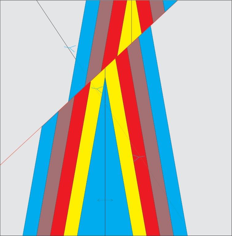
Step 5: Unconstrained interpretation

If additional data are known, such as the position of a syncline on the surface or from another drill hole, the reconstruction can continue to infill around this position.

Step 6: Speculative interpretation & target generation

We may be able to hypothesis structures that may infill the blanks. Using representative structural styles seen in the region, these can be hypothesised and drawn in to propose new drill targets to test.

This is where the true value of the interpretive process lies for the explorer. The ability to see into the unknown and define new targets but built from the solid foundations of their reconstructed and interpreted data.